Once on a wonderful Berlin winter day more than a year ago I was thinking of nothing evil when suddenly…

Bugsnag popped up and complained about an
Elixir.DBConnection.ConnectionError - I took a look immediately to find out
what made our wonderful application crash. It turned out
it was a timeout error! Ecto (elixir database tool) defaults to a timeout of 15
seconds and we
had a query that took longer than this? Yikes! What happened?
This is the story of what happened, where we went wrong and how we made sure we fixed it.
The problem
The application we are looking at here is our courier tracker. It gets the GPS locations of couriers on the road and then makes them available for admins to look at through websockets. One important part of this is that as soon as you look at a shipment its last known location is displayed. This was where the exception was raised:
last_courier_location =
  LatestCourierLocation
  |> CourierLocation.with_courier_ids(courier_id)
  |> Repo.one
How could this innocent line take so long (remember the query took 15 seconds to execute) and what does it do?
with_courier_ids/2 basically resolves to this:
def with_courier_ids(query, courier_ids) when is_list(courier_ids) do
  from location in query,
  where: location.courier_id in ^courier_ids
end
Instead of a straight id = my_id check it checks against the inclusion in a list
(the list being [courier_id] on the Elixir side).
LatestCourierLocation on the other hand is a
database view
that we created as follows:
CREATE OR REPLACE VIEW latest_courier_locations AS
  SELECT DISTINCT ON(courier_id)
  *
  FROM courier_locations
  ORDER BY courier_id, time DESC
So it does what we said in the beginning–it gets the latest location for a given courier. Easy enough.
Why did it take so long?
A quick debugging showed that it took so long because a misbehaving client was submitting locations at a way too frequent rate. At the time, that courier had around 2.5 million locations in the database. That’s quite a lot, but nothing that should cause the database to take that long.
This is probably also a good time to mention that we are running PostgreSQL 9.6 along with ecto 2.1.6 and postgrex 0.13.3.
First Attempt
OK, let’s make this faster. I got this. I know this. Let’s write a benchmark! Benchmarking is done on a production-like database minus the sensitive data so that our results will translate to the production environment. We’ll use benchee:
alias CourierTracker.{Repo, CourierLocation, LatestCourierLocation}
require Ecto.Query

courier_id = 3799 # this courier has about 2.5 million locations in my db

Benchee.run %{
  "DB View" => fn ->
    LatestCourierLocation
    |> CourierLocation.with_courier_ids(courier_id)
    |> Repo.one(timeout: :infinity)
  end,
  "with_courier_ids" => fn ->
    CourierLocation.with_courier_ids(courier_id)
    |> Ecto.Query.order_by(desc: :time)
    |> Ecto.Query.limit(1)
    |> Repo.one(timeout: :infinity)
  end,
  "full custom" => fn ->
    CourierLocation
    |> Ecto.Query.where(courier_id: ^courier_id)
    |> Ecto.Query.order_by(desc: :time)
    |> Ecto.Query.limit(1)
    |> Repo.one(timeout: :infinity)
  end
}, time: 30,
   warmup: 5,
   formatters: [
     &Benchee.Formatters.Console.output/1,
     &Benchee.Formatters.HTML.output/1
   ],
   html: [file: "benchmarks/reports/latest_location_single.html"]
What does this do? It defines 3 variants that we want to benchmark (DB View,
with_courier_ids and full customer) along with the code that should be
measured. We measure this with the specific id that was causing the error.
We then also define a warmup period of 5 seconds and a measurement time of 30 seconds for each of the defined jobs. We also say we want to output this in the console as well as in an HTML format (this allows png exports).
So what does the benchmark say?
tobi@liefy ~/projects/liefery-courier-tracker $ mix run benchmarks/latest_location_no_input.exs
Operating System: Linux
CPU Information: Intel(R) Core(TM) i7-6700HQ CPU @ 2.60GHz
Number of Available Cores: 8
Available memory: 15.49 GB
Elixir 1.4.5
Erlang 20.1
Benchmark suite executing with the following configuration:
warmup: 5 s
time: 30 s
parallel: 1
inputs: none specified
Estimated total run time: 1.75 min


Benchmarking DB View...
Benchmarking full custom...
Benchmarking with_courier_ids...

Name                 ips     average  deviation      median      99th %
with_courier_ids  983.21     1.02 ms    ±43.22%     0.91 ms     3.19 ms
full custom       855.07     1.17 ms    ±53.86%     0.96 ms     4.25 ms
DB View             0.21  4704.70 ms     ±4.89%  4738.83 ms  4964.49 ms

Comparison:
with_courier_ids  983.21
full custom       855.07 - 1.15x slower
DB View             0.21 - 4625.70x slower
It says a lot of things, but first of all it mentions what system the benchmark was run on. So, if you’re interested in the CPU, elixir or erlang version… they’re all right there!
But what do the results say? Apparently with_courier_ids and full custom
rock! DB View is over 4600 times slower!. Wow case solved. Using a nice
visual representation from the HTML report makes this even clearer:
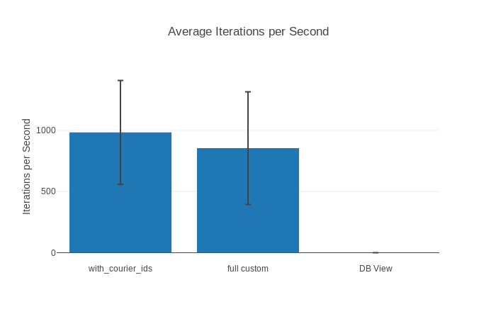
(displayed is how many iterations we could do per second on average, so bigger is better!)
The standard deviation seems sort of high (~10% would be more normal) but our worst case performance (99th%) is still under 5 ms so we seem to be good.
This should be enough. So, let’s switch our our current implementation
(DB View) with the most performant one from the benchmark
(with_courier_ids). Commit it, push it, merge it, roll it out, pat ourselves
on the back for one of the best performance improvements ever and call it a day!
Boom!
We deploy and boom…

The bugsnag errors start rolling in! Look at all these DBConnectionErrors! There are
more than before! How? We benchmarked this! This can’t be happening!
No time to argue with reality. Let’s rollback these changes and investigate.
What happened?
Taking a look at the logs we find out that the new errors happened when the courier we were requesting locations for had no locations at all or fairly fe. This can happen when the feature is turned off or the courier doesn’t use our app.
Ok then, let’s write a new benchmark! This time we’ll use a wider range of
inputs. Luckily benchee has us covered with the
inputs feature:
# in benchmarls/latest_location.exs or some such file
alias CourierTracker.{Repo, CourierLocation, LatestCourierLocation}
require Ecto.Query

# Use the ids of couriers that have a certain amount of locations in my db
inputs = %{
  "Big 2.5 million locations" => 3799,
  "No locations"              => 8901,
  "~200k locations"           => 4238,
  "~20k locations"            => 4201
}

Benchee.run %{
  "DB View" => fn(courier_id) ->
    LatestCourierLocation
    |> CourierLocation.with_courier_ids(courier_id)
    |> Repo.one(timeout: :infinity)
  end,
  "with_courier_ids" => fn(courier_id) ->
    CourierLocation.with_courier_ids(courier_id)
    |> Ecto.Query.order_by(desc: :time)
    |> Ecto.Query.limit(1)
    |> Repo.one(timeout: :infinity)
  end,
  "full custom" => fn(courier_id) ->
    CourierLocation
    |> Ecto.Query.where(courier_id: ^courier_id)
    |> Ecto.Query.order_by(desc: :time)
    |> Ecto.Query.limit(1)
    |> Repo.one(timeout: :infinity)
  end
}, inputs: inputs, time: 30, warmup: 5,
   formatters: [
     &Benchee.Formatters.Console.output/1,
     &Benchee.Formatters.HTML.output/1
   ],
   html: [file: "benchmarks/reports/latest_location.html"]
I’ll spare you the output of system metrics etc. this time around. Let’s have a look at the results divided by input:
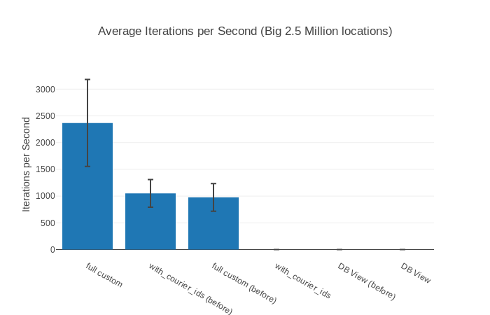
##### With input Big 2.5 million locations #####
Name ips average deviation median 99th %
with_courier_ids 937.18 1.07 ms ±34.98% 0.95 ms 2.64 ms
full custom 843.24 1.19 ms ±52.82% 0.99 ms 4.37 ms
DB View 0.22 4547.24 ms ±2.80% 4503.63 ms 4718.76 ms
Comparison:
with_courier_ids 937.18
full custom 843.24 - 1.11x slower
DB View 0.22 - 4261.57x slower
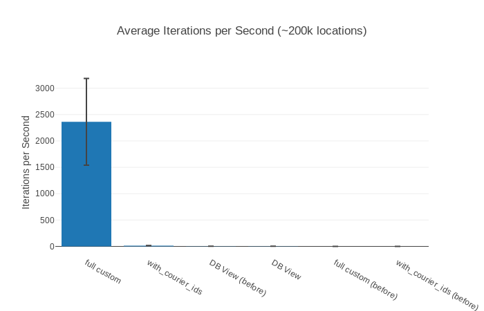
##### With input ~200k locations #####
Name ips average deviation median 99th %
DB View 3.57 0.28 s ±7.84% 0.28 s 0.35 s
with_courier_ids 0.109 9.19 s ±2.25% 9.13 s 9.53 s
full custom 0.0978 10.23 s ±0.95% 10.23 s 10.34 s
Comparison:
DB View 3.57
with_courier_ids 0.109 - 32.84x slower
full custom 0.0978 - 36.53x slower
##### With input ~20k locations #####
Name ips average deviation median 99th %
DB View 31.73 0.0315 s ±12.50% 0.0298 s 0.0469 s
with_courier_ids 0.104 9.62 s ±0.84% 9.59 s 9.76 s
full custom 0.0897 11.14 s ±1.38% 11.17 s 11.32 s
Comparison:
DB View 31.73
with_courier_ids 0.104 - 305.37x slower
full custom 0.0897 - 353.61x slower
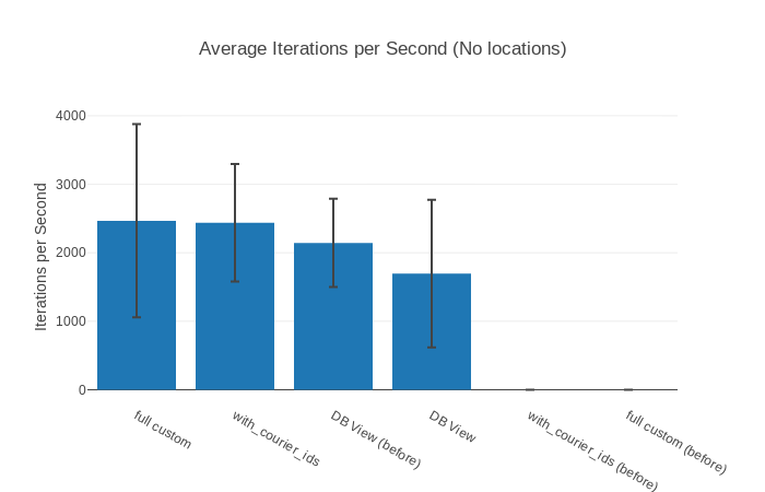
##### With input No locations #####
Name ips average deviation median 99th %
DB View 1885.48 0.00053 s ±44.06% 0.00047 s 0.00164 s
with_courier_ids 0.0522 19.16 s ±3.77% 19.16 s 19.88 s
full custom 0.0505 19.82 s ±1.58% 19.82 s 20.13 s
Comparison:
DB View 1885.48
with_courier_ids 0.0522 - 36123.13x slower
full custom 0.0505 - 37367.23x slower
It seems like DB View is faster than our 2 alternatives for everything that
doesn’t have the 2.5 million locations? And not just by a little bit,
for no locations our “faster” alternatives are more than
35 000 times slower! How can this be? full custom and
with_courier_ids get slower the fewer locations their respective couriers
have?
To find out what’s going on, let’s get the respective queries, fire up a
PostgreSQL shell and EXPLAIN ANALYZE what’s up. It’s basically asking
PostgreSQL (or the query planner, more precisely) how it wants to get that data.
Seeing that, we might find out where we are missing an index or where our data
model hurts us.
To get the SQL query each one of our possibilities would generate, we can use
Ecto.Adapters.SQL.to_sql/3.
Let’s use it:
iex(1)> query = CourierLocation |> Ecto.Query.where(courier_id: 3799)
|> Ecto.Query.order_by(desc: :time) |> Ecto.Query.limit(1)
#Ecto.Query<from c in CourierTracker.CourierLocation,
 where: c.courier_id == 3799, order_by: [desc: c.time], limit: 1>
iex(2)> {string, _args} = Ecto.Adapters.SQL.to_sql(:all, Repo, query)
{"SELECT c0.\"id\", c0.\"courier_id\", c0.\"location\", c0.\"time\",
c0.\"accuracy\", c0.\"inserted_at\", c0.\"updated_at\"
FROM \"courier_locations\" AS c0 WHERE (c0.\"courier_id\" = 3799)
ORDER BY c0.\"time\" DESC LIMIT 1", []}
iex(3)> IO.puts string
SELECT c0."id", c0."courier_id", c0."location", c0."time", c0."accuracy",
c0."inserted_at", c0."updated_at"
FROM "courier_locations" AS c0
WHERE (c0."courier_id" = 3799)
ORDER BY c0."time" DESC LIMIT 1
:ok
We can just take the string we printed out and copy & paste it into a psql
console. Let’s first check out full custom (reformatted for readability):
courier_tracker=# EXPLAIN ANALYZE
  SELECT c0."id",
         c0."courier_id",
         c0."location",
         c0."time",
         c0."accuracy",
         c0."inserted_at",
         c0."updated_at"
   FROM "courier_locations" AS c0
  WHERE (c0."courier_id" = 3799)
  ORDER BY c0."time" DESC LIMIT 1;

                                 QUERY PLAN
--------------------------------------------------------------------------------
 Limit  (cost=0.43..0.83 rows=1 width=72)
        (actual time=1.840..1.841 rows=1 loops=1)
   ->  Index Scan Backward using courier_locations_time_index on
       courier_locations c0
       (cost=0.43..932600.17 rows=2386932 width=72)
       actual time=1.837..1.837 rows=1 loops=1)
         Filter: (courier_id = 3799)
         Rows Removed by Filter: 1371
 Planning time: 0.190 ms
 Execution time: 1.894 ms
(6 rows)
What does this tell us? It uses the index on time to efficiently order the
courier locations by time to get the most recent one for a given courier.
That works brilliantly if there is a recent one. If there is no recent one we’ll
still scan the whole table until we realize there isn’t any 😱😱😱
That explains why full custom is slower the fewer locations we have (the
lower our chances to hit a recent location of a given courier, basically).
with_courier_ids is much the same.
What does DB View do differently?
courier_tracker=# EXPLAIN ANALYZE
SELECT l0."id",
       l0."courier_id",
       l0."location",
       l0."time",
       l0."inserted_at",
       l0."updated_at"
  FROM "latest_courier_locations"
    AS l0
 WHERE (l0."courier_id" = ANY('{3799}'));

                                  QUERY PLAN
------------------------------------------------------------------------------
 Unique  (cost=650416.51..662351.17 rows=282 width=64)
          (actual time=3135.211..3969.453 rows=1 loops=1)
   ->  Sort  (cost=650416.51..656383.84 rows=2386932 width=64)
             (actual time=3135.211..3849.342 rows=2508672 loops=1)
         Sort Key: courier_locations.courier_id, courier_locations."time" DESC
         Sort Method: external merge  Disk: 181472kB
         ->  Bitmap Heap Scan on courier_locations
             (cost=44683.16..218073.14 rows=2386932 width=64)
             (actual time=179.249..601.531 rows=2508672 loops=1)
               Recheck Cond: (courier_id = ANY ('{3799}'::integer[]))
               Heap Blocks: exact=33490
               ->  Bitmap Index Scan on courier_locations_courier_id_index
                   (cost=0.00..44086.42 rows=2386932 width=0)
                   (actual time=172.958..172.958 rows=2508672 loops=1)
                     Index Cond: (courier_id = ANY ('{3799}'::integer[]))
 Planning time: 0.344 ms
 Execution time: 3992.065 ms
(11 rows)
Our biggest time investment here is the sorting by time (without an index!) that
PostgreSQL performs, scanning is then done by the index on courier_id.
Most likely this goes back to the way we defined the database view.
The sort is cheaper the fewer locations are affected (which we find efficiently
in this case) - explaining how it is faster for those compared to
full custom & friends.
So, what’s the solution? Our attempts seem to use either the index on
courier_id or the index on time - if only there was a way to combine
them…
Combined Indexes to the rescue

We can define indexes on
multiple columns
and it’s importat that the most limiting index is the leftmost one. As we
usually scope by couriers, we’ll make courier_id the left most.
So let’s migrate our database!
defmodule CourierTracker.Repo.Migrations.LongLiveTheCombinedIndex do
  use Ecto.Migration

  def change do
    drop index(:courier_locations, [:courier_id])
    drop index(:courier_locations, [:time])
    create index(:courier_locations, [:courier_id, :time])
  end
end
As our combined index can basically be used as a replacement for the leftmost
index (courier_id) and we learned we
don’t want to scan only based on time it is safe to drop those.
But how do we know that we improved on our old results? We could just run the
benchmarks again and compare by hand… or we could use benchee’s new feature
introduced in 0.12 for
saving, loading and comparing previous runs!
It’s easy to use. Just add save: [tag: "before", path: "location.benchee"] to the
configuration and run it again before we run the migration to save the “before”
results. Then we run the migration, set load: "location.benchee" in the
benchmark to load them up again and compare against the old results.
Well I’ve given you enough plain text to read for one day haven’t I? Let’s just
go with the images for now. If the details (including histograms, raw runtime
graphs & more) interest you feel free to check out the
full HTML report.
Suffice it to say, full custom with a combined index is now the fastest with
all inputs.
Results from before our migration to combined indexes are annotated as (before).
2.5 million Locations
200 000 Locations
20 000 locations

No Locations
The Query Plan
How has our query plan changed now that we use a combined index you might ask,
well here you go (for full custom):
courier_tracker=# EXPLAIN ANALYZE
  SELECT c0."id",
         c0."courier_id",
         c0."location",
         c0."time",
         c0."accuracy",
         c0."inserted_at",
         c0."updated_at"
   FROM "courier_locations" AS c0
  WHERE (c0."courier_id" = 3799)
  ORDER BY c0."time" DESC LIMIT 1;

                                 QUERY PLAN
--------------------------------------------------------------------------------
 Limit  (cost=0.43..2.94 rows=1 width=72) (actual time=0.047..0.048 rows=1 loops=1)
   ->  Index Scan Backward using courier_locations_courier_id_time_index on
       courier_locations c0
       (cost=0.43..273924.89 rows=109445 width=72)
       (actual time=0.045..0.045 rows=1 loops=1)
         Index Cond: (courier_id = 3799)
 Planning time: 0.255 ms
 Execution time: 0.108 ms
(5 rows)
It looks much like our previous query plan (save the changed index name),
however notice how instead of Filter: (courier_id = 3799) it says Index Cond:
(courier_id = 3799)? That’s the index kicking in!
One more thing
I know it’s time to wrap this up already, but there’s one more important thing! When you add indexes etc. it’s always wise to also benchmark the time it takes you to insert records into the database. A simple benchmark:
alias CourierTracker.{Repo, CourierLocation}

valid_location = %{
  courier_id: 42,
  location: %Geo.Point{coordinates: {1.0, 42.0}},
  time: "2010-04-17T14:00:00Z"
}

Benchee.run %{
  "Inserting a location" => fn ->
    changeset = CourierLocation.changeset(%CourierLocation{}, valid_location)
    Repo.insert!(changeset)
  end
}, load: "insertion.benchee"#, save: [tag: "old", path: "insertion.benchee"]
And the result:
Name                           ips  average  deviation   median   99th %
Inserting a location (old)  353.46  2.83 ms    ±20.58%  2.69 ms  4.88 ms
Inserting a location        348.17  2.87 ms    ±42.25%  2.37 ms  7.92 ms

Comparison:
Inserting a location (old)  353.46
Inserting a location        348.17 - 1.02x slower
That’s the same-ish difference and could easily be explained by the deviation. So, we’re good.
Takeaway
What did this journey teach us in the end?
Always benchmark with a variety of inputs! Even if you think your input is definitely the worst case, it’s you guessing–not knowing. Algorithms and systems often have interesting worst cases. The results might surprise you, as they surprised me here.
Obviously we should have also noticed this slow query earlier by using application performance monitoring. Back then there weren’t very many good tools for this, and our application had never caused us any problems. Now, however, there’s some great tools out there.
So, take your trusty benchmarking tool and remember your inputs. Then, you too can have a nice comfortable house… errm application again.